


Introduction
Deep learning and machine learning models are fundamentally collections of mathematical functions. They transform inputs, like a question in a language model, into outputs, such as a generated sentence or image. To refine the accuracy of these models, we need a way to adjust their internal parameters. This adjustment process relies heavily on understanding how parameter changes affect the model's output, which is quantified by a "loss function".
The core concept that allows us to understand these changes is the derivative. Derivatives, as you may recall from your math class, describe the rate of change of a function. We can determine these derivatives through direct calculation in code or by using approximations. However, deep learning often utilizes a technique called automatic differentiation (AD). This method provides a systematic way to compute derivatives of complex functions, which are essential for adjusting the model's parameters. In this blog post, I will delve into AD and its implementation within a Haskell library, focusing on how it enables the computation of derivatives without discussing the broader concept of parameter adjustment or optimization.
This blog post assumes that you are familiar with:
- Calculus concepts: Derivatives, Jacobians, chain rule of differentiation, gradients. (I would also recommend going through the 3Blue1Brown video series as a good start)
- Haskell and programming in general.
The foundation of AD is the concept that a computational graph can represent both the value of a function and its derivatives. This graph deconstructs the function into a series of elementary operations (i.e, addition, division), each represented by a node. These nodes store intermediate values and their derivatives, which are computed using the chain rule. The two primary modes of AD are forward mode and backward mode.
Forward Mode AD
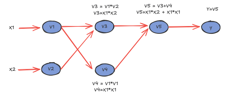
This is the simplest way of calculating the derivative of a multivariable function. Consider the following function, which takes two independent variables x1, x2, and has one dependent variable y=f(x1,x2).
f(x1,x2) = x1 * x2 + x1²
The forward mode AD calculates the derivative by traversing the graph for each of the independent variables by calculating derivatives of each vi partial function by considering the following for a given independent variable x1:
v̇i = ∂vi/∂x 1
For example, to calculate the derivative x1 at point x1=2 and x2=3, the algorithm traverses the graph and evaluates the function and its derivative:
| Intermediate variables | Forward evaluation | Forward differentiation | Evaluation of the derivative |
|---|---|---|---|
| V1 = X1 | = 2 | v̇1 = ẋ1 | = 1 |
| V2 = x2 | = 3 | v̇2 = ẋ2 | = 0 |
| V3 = V1 * V2 | = 2*3 = 6 | v̇3 = v̇1 * v2 + v̇2 * v1 | =1 * 3 + 0 * 2= 3 |
| V4 = V1 * V1 | = 2*2 = 4 | v̇4 = ẋ1 * v1 + v1 * v̇1 | = 1 * 2 + 2 * 1=4 |
| V5 = V3 + V4 | = 6 + 4= 10 | v̇5 = v̇3 + v̇4 | = 3 + 4 = 7 |
| Y = V5 | = 10 | dy/dx1 = v̇5 | = 7 |
Forward Automatic Differentiation is inappropriate for machine learning optimization (check this article) due to its inefficiency in calculating the gradient for scalar functions with multiple independent variables. In such cases, multiple graph traversals are necessary, making Reverse mode Automatic Differentiation a more suitable choice.
There is another way to compute derivatives on Forward mode by using a special number called Dual Number. However, the use of a Dual Number is out of the scope of this post.
Reverse mode AD
The reverse mode automatic differentiation is calculated in two phases: The first phase calculates each of the intermediate values vi and records them in the computational graph. The second phase, referred to as backpropagation, calculates the derivatives by considering the adjoints of vi from the outputs to the inputs. The adjoints are defined as follows:
V̄i =∂y/∂v i
So, we're looking at how sensitive the current output is to changes in each vi. Adjoints show how much each vi contributes to the change in the output of the function f(X). During backpropagation, we start with the derivative of the function with respect to itself, which is 1.
The following table shows an example of reverse mode AD, by considering the same function as before.
| Intermediate variables | Forward evaluation (Top down) | Backward differentiation (Bottom up) | Derivatives |
|---|---|---|---|
| V1 = X1 | = 2 | V̄1 = ∂y/∂x1 =V̄3 * ∂v3/∂v1 + V̄4 * ∂v4/∂v1 = 1 * x2 + 1 * 2 * x1 |
= x2 + 2x1 |
| V2 = x2 | = 3 | V̄2 = ∂y/∂x2 = V̄3 * ∂v3/∂v2 = V̄5 * (x1) = x1 |
= x1 |
| V3 = V1 * V2 | = 2*3 = 6 | V̄3 = ∂y/∂v3 = ẋ5 * ∂v5/∂v3 = V̄5 * 1 | = 1 |
| V4 = V1 * V1 | = 2*2 = 4 | V̄4 = ∂y/∂v4 = V̄5 * ∂v5/∂v4 = V̄5 * ∂(v3 + v4)/∂v4 = V̄5 |
= 1*1=1 |
| V5 = V3 + V4 | = 6 + 4 = 10 | V̄5 = ∂y/∂v5 = ȳ * ∂y/∂v5 = ȳ | = 1*1=1 |
| Y = V5 | = 10 | ȳ = ∂y/∂v5 | = 1 |
Take a look at V̄1. Going back to the computational graph we see that v1 contributes to both v3 and v4 and that's why we need to sum their respective derivatives with respect to v1. Now if we evaluate ∂y/∂x1 withx1=2 and x2=3 we get the value of 7, the same value we calculated with forward mode AD.
In summary, Reverse mode AD can be defined with the following steps:
- The forward phase evaluation to get the function evaluation for the given inputs.
- The reverse phase starts with
ȳ=1and visits each of the parent nodes. - For each parent node
vi: calculate the contributionV̄iof the change in eachvito the change in the output y. - At the end of the reverse mode you get the partial derivatives of the function with respect to each independent variable.
The AD Haskell library
Everything above was the theory behind Automatic differentiation. We now switch to Haskell and a library that implements this paradigm. The name is just ad, and at the time of writing this post, the latest release is 4.5.6 and has 376 stars on GitHub. This library offers a set of modules to compute derivatives (gradients, jacobians, directional derivatives and Hessians) by using either Reverse or Forward mode.
The core of this library is that each mode is represented by types and typeclasses; for example, AD and its forward mode have the following definitions:
newtype AD s a = AD { runAD :: a }
  deriving (Eq,Ord,Show,Read,Bounded,Num,Real,Fractional,Floating,Enum,RealFrac,RealFloat,Erf,InvErf,Typeable)

data Forward a
  = Forward !a a
  | Lift !a
  | Zero
  deriving (Show, Data, Typeable)
Take a look at the first constructor, (Forward !a a). The first argument is the value of the function evaluation and the second is its accumulative derivative (da).
The reverse mode is defined as follows:
data Reverse s a where
  Zero :: Reverse s a
  Lift :: a -> Reverse s a
  Reverse :: {-# UNPACK #-} !Int -> a -> Reverse s a
  deriving Show
And each mode is represented by a typeclass:
class (Num t, Num (Scalar t)) => Mode t where
  type Scalar t
  type Scalar t = t

  -- | allowed to return False for items with a zero derivative, but we'll give more NaNs than strictly necessary
  isKnownConstant :: t -> Bool
  isKnownConstant _ = False

  asKnownConstant :: t -> Maybe (Scalar t)
  asKnownConstant _ = Nothing

  -- | allowed to return False for zero, but we give more NaN's than strictly necessary
  isKnownZero :: t -> Bool
  isKnownZero _ = False

  -- | Embed a constant
  auto  :: Scalar t -> t
  default auto :: (Scalar t ~ t) => Scalar t -> t
  auto = id

  -- | Scalar-vector multiplication
  (*^) :: Scalar t -> t -> t
  a *^ b = auto a * b

  -- | Vector-scalar multiplication
  (^*) :: t -> Scalar t -> t
  a ^* b = a * auto b

  -- | Scalar division
  (^/) :: Fractional (Scalar t) => t -> Scalar t -> t
  a ^/ b = a ^* recip b

  -- |
  -- @'zero' = 'lift' 0@
  zero :: t
  zero = auto 0
Computing gradients with the AD library
Given the above function that we used for our manual examples, we can compute the gradient for the same inputs by using the grad function from the library. The following code snippet, shows the type signature and an example of computing the gradient with Forward mode:
ghci> :t grad
grad
  :: (Traversable f, Num a) =>
    (forall s. f (AD s (Forward a)) -> AD s (Forward a)) -> f a -> f a
ghci> import Numeric.AD.Mode.Forward
ghci> grad (\[x1,x2]-> x1*x2 + x1*x1) [2,3]
[7,2]
ghci>
It takes:
- The function that we want to compute the gradient for any given mathematical function:
(forall s. f (AD s (Forward a)) -> AD s (Forward a)).
- The values where the gradient would be evaluated:
f a
And returns the gradient in the context f a: [7,2] which is the gradient evaluated at [2,3].
There is also a grad function that implements the reverse mode. In the following code snippet, we can see that it has almost the same type signature as the forward mode version:
ghci> import Numeric.AD.Mode.Reverse
ghci> :t grad
grad
  :: (Traversable f, Num a) =>
    (forall s.(Reifies s Tape,Typeable s) =>f (Reverse s a) -> Reverse s a)
    -> f a
-> f a
ghci> grad (\[x1,x2]-> x1*x2 + x1*x1) [2,3]
[7,2]
ghci>
I recommend that you examine the library's additional differentiation functionalities and empirically evaluate the performance of both the forward and backward modes.
Summary and key points:
Automatic differentiation is really powerful when it comes to calculating derivatives for a function. Deep learning libraries like PyTorch (see autograd) and Tensorflow (see GradientTape) implement this paradigm to optimize deep learning models and adjust their parameters to allow them to learn from data. The Haskell AD library offers the implementation of this paradigm for both modes and has functions to calculate gradients, jacobians, directional derivatives, and Hessians by implementing a common API for each mode.
This blog post outlines the fundamentals of Automatic Differentiation. Below is a curated list of valuable resources for those interested in further exploration.
- Automatic differentiation in machine learning: a survey: This has a good explanation of why Reverse Mode is used in Machine Learning.
- What's Automatic Differentiation?
- Automatic Differentiation Background
- Basic Parameter Estimation, Reverse-Mode AD, and Inverse Problems: This has examples of Reverse mode AD with logistic regression and a Neural Network
- Deep into Deep Learning Chapter 2.5: Automatic Differentiation.
- Reverse-mode automatic differentiation from scratch, in Python